
[ad_1]
This may get a little math-y, but please bear with me. I’ll try to keep it (as Einstein would say) “as simple as possible, but not simpler”.
Start with sound waves that come from an orchestra. The pressure on your eardrum goes up and down many times per second in a pattern that looks chaotic to the eye.
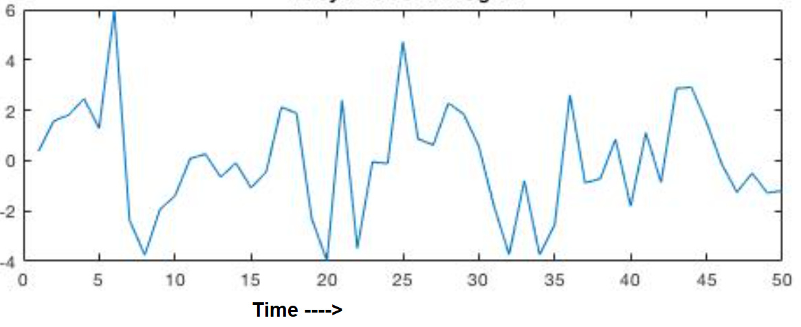
This is the raw signal that the ear is receiving, but the ear hears musical notes! Tiny hairs in the ear are tuned each to a different frequency, and pick up just that part of the signal that is (for example) an E flat above middle C on the piano.
What the ear does mechanically can also be done with mathematics. The procedure was discovered by Jean-Baptiste (“Joe”) Fourier and first published in 1822. The procedure involves a great deal of arithmetic, though it can be written in a very compact notation using integral calculus. You don’t have to understand anything about the procedure except that it’s called a Fourier Transform, and it turns that pressure function — how strong was the pressure at each moment of time — into another function that tells you how much of each musical note was present in the sound that the ear heard.
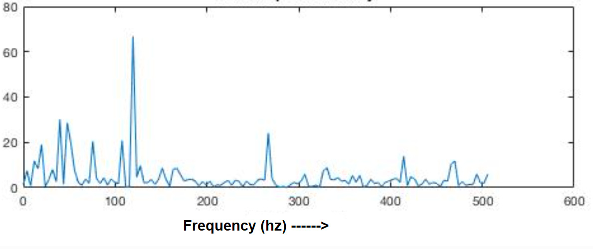
A natural question to ask is about when each note was played by the orchestra. The Fourier transform contains this information as well. It is treated as a very low frequency. For example, the orchestra may play 5 notes C D E F G in a single second. The ear hears this as five different notes in a rhythmic sequence. To the ear, the time scale of hundredths of a second defines the note, but the time scale of tenths of a second is heard as separate notes. But to the Fourier transform, these two time scales are part of a continuum. The Fourier transform treats tenths of a second and hundredths of a second with the same mathematics. The result is that the Fourier transform contains information about which notes are played and also when they are played, all coded in the same mathematical function.
These two graphs, the two functions contain exactly the same information. They are different mathematical descriptions, but they correspond to exactly the same physical situation. Both are ways of describing the sound waves that impinge on your ear.
We know that they have the same information because you can perform this mathematical trick, the Fourier transform, and convert the pressure representation into the notes-of-the-scale representation. (A physicist would call the former the “time domain” and the latter the “frequency domain”.)
The Fourier transform converts the graph in the time domain to a graph in the frequency domain. If they really contain the same information, it should be possible to perform another mathematical procedure, call it the “inverse Fourier transform”, and convert the frequency domain back to the time domain. The inverse transform allows you to recover the first graph from the second graph.
“Joe” had this all worked out. The Fourier transform converts the time graph to the frequency graph. The Inverse Fourier transform converts the frequency graph back to the time graph.
Now comes the mathemagic that must have surprised and delighted Joe, even as it surprises and delights physics students 200 years later.
The Fourier Transform and the Inverse Fourier Transform are exactly the same. Whatever you do to the first graph to get the second graph can also be done to the second graph and, lo and behold, you get back the first graph.
Remember, the Fourier Transform is an intricate recipe involving oodles of arithmetic that you perform on the numbers that make up the first graph. When you follow this recipe, you end up with the second graph. Now if you take the second graph and you apply the same recipe, you get back the first graph.
The same Fourier Transform, applied twice, takes you right back to the original graph that you started with.
The lesson we’ve learned so far is that the same information is contained in these two graphs. The two graphs are equivalent ways of describing a single physical situation. Either description will do.
Here’s an example that we’ll come back to later. Suppose the orchestra is on strike, and one man comes out on stage with a tuning fork tuned to A 440. He plays a single note. The graph #1, pressure on the ear, is a sine wave. It looks like this.
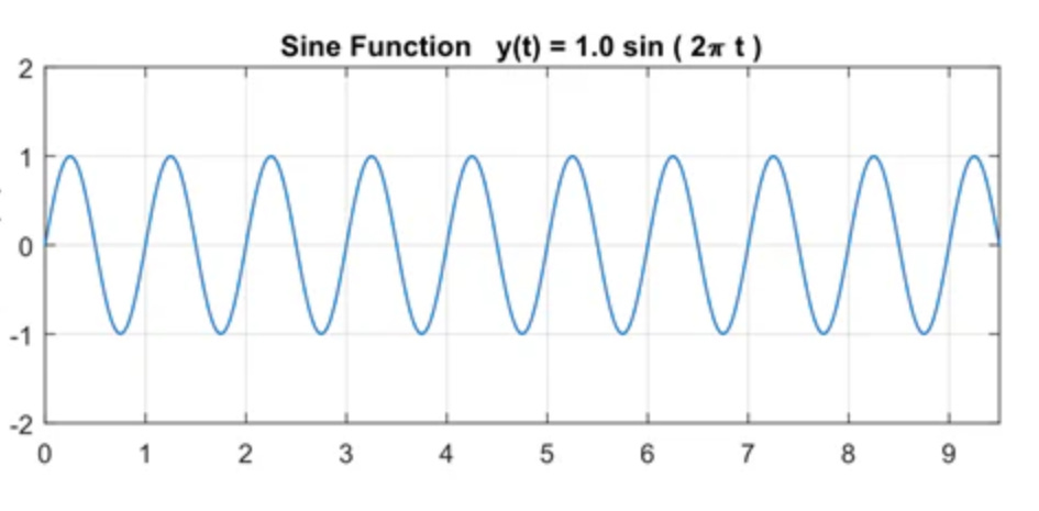
What does graph #2 look like? For every note that’s not A 440 the contribution is zero. So graph #2 is zero everywhere except for a sharp spike at A 440.
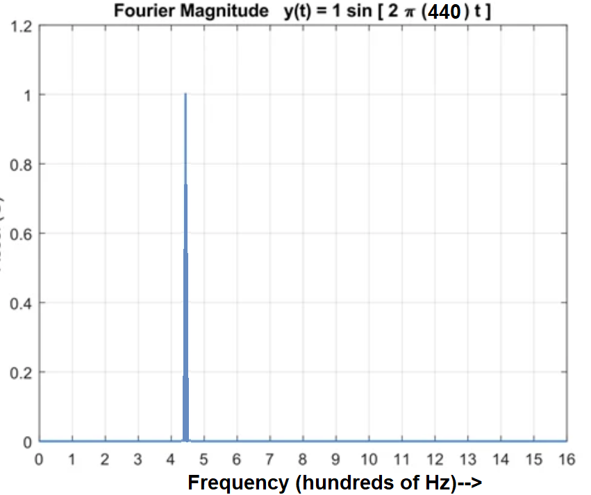
I’ve drawn a wedge, but I ask you to imagine that the spike at A440 is infinitely thin.
Can we Fourier transform this spike back to get the sine wave? Here’s trick that should work: We know this spike is in frequency space, but we said that the same Fourier math works forward or backward. It shouldn’t matter if it’s in frequency space or it’s pressure-vs-time. So let’s imagine the spike is in time. It looks like a big pressure pulse at one time, with nothing before or after. There is a pulse of sound at just one moment, like a bang or a clap or a click. The Fourier transform of that should look like a graph of what frequencies are present in a clap. The ear doesn’t hear any particular frequency, and the answer is that all frequencies are contributing equally. So when we Fourier transform the clap we get a constant function, a line that is the same everywhere.
Woops — we were expecting to get back the sine wave. What happened? The two are sort of alike, in that they spread evenly, but one is wavy and the other is straight.
The answer is that I cheated you when I said that the Fourier transform is just a recipe for a lot of arithmetic operations on the numbers in graph #1. The graph is just an ordinary plot of real numbers. What I didn’t tell you is that, for it all to work out as I said, the numbers have to be complex numbers, two-part numbers, real and imaginary, a + bi.
Now that I’ve said this, I ask you to leave it in the back of your mind. It doesn’t matter for much of follows. I’ll let you know if you need to think about imaginary numbers, and mostly you won’t.
Aside: Fourier and Holograms
Where is the information? The pressure on your eardrum at every point in time depends on all the different notes that are being played, because they combine together.
This may remind you of the way a hologram works. You can turn a photograph into a hologram, and every point on the hologram contains information about the whole photo. A laser beam can create a hologram from the photo, and the same laser beam can re-create the photo from the hologram.
The similarity is not a coincidence. A hologram is a Fourier transform in two dimensions.
I hope I’ve convinced you that the sound wave is one thing, and you can represent it either in the frequency domain or in the time domain. Either one contains the same information. Hold that thought as we move on to quantum physics.
In acoustics, Joe Fourier’s math works for us, giving us two ways we can look at any situation. We can take our pick, and work with whichever whichever representation is more convenient. But in quantum mechanics, Joe’s math works against us. It’s the same math, but it’s no longer about two different representations of the same thing. It’s about two different things, and we need both of them but Joe tells us we can only have one at a time. This is the story coming up.
Think of a billiard ball bouncing around a table. If I want to know everything about how that ball is moving, all I need is two pairs of numbers.
Pick a time, any time. The first pair of numbers tells me where the ball is. We can think of the x and y coordinates that define the ball’s position at your chosen time. The other thing we need to know is how fast the ball is moving, and in what direction. That’s another pair of numbers, that we can think of as a speed and an angle, or else, just as good, we could get the same information from its velocity in the x direction vx and velocity in the y direction vy.
Once we know (x, y) and (vx , vy), we know all there is to know about the situation. We can follow the billiard ball around the table. We can know where it is going to be and how fast it is moving at any time in the future.
It’s not enough to know (x, y) or (vx , vy) separately. We need to know both the position and the velocity at any one time. Then we have all the information we need to calculate the ball’s trajectory forever after.
With this foundation, we’re ready for one of the great paradoxes of quantum physics. In QM, we’re not working with the exact position of the billiard ball. Instead we have a “wave function” that tells us the probability of the the billiard ball being at a given place on the green table. The wave function associates a probability with every point on the table. If the wave function is small around the edges and large in the center, that means that there’s a high probability that the ball is near the center of the table.
Now we’re ready to bring in the Fourier math. Here’s a profound truth that Neils Bohr bequeathed to us: There’s a wave function for the position of the ball, as we just described. The position wave function tells you the probability the ball will be found at any given location. There’s also a wave function for the velocity of the same ball. The velocity wave function tells you the probability of the ball having any given velocity.
The velocity wave function is the Fourier transform of the position wave function.
If this doesn’t make any sense to you, then you’re understanding something important. We want to know where the ball is, and QM tells us we can’t know it exactly. We can only know a probability distribution. OK we can live with that. Now, we also want to know the velocity of the ball. And Bohr is telling us that this is not a separate probability distribution. It’s already determined when we specified the probability distribution for the ball’s location.
Bohr called it “complementarity”, but having a name for it doesn’t make it any more sensible.
Make this practical. Say we pin down the ball in the center of the table. We know exactly where it is. So its wave function is a thin spike, as we described above for the sound of a clap.
The radical dictate of the Complementarity Principle tells us that we don’t have to measure the ball’s velocity. We already know all that can be known about it, and that is the velocity wave function. The velocity wave function is the Fourier transform of the position wave function. Above, we did that exercise — we said that a clap has no particular sound frequency, so it contains equal amounts of all frequencies. The Fourier transform of the spike is the constant function, the same everywhere.
Translate the math to physics, and we get this very inconvenient, very unwelcome limitation. When we know the exact position of the ball, its velocity is as unknown as it can be. It has the same probability of going fast or slow, of going left or right or backwards or forwards. The velocity is completely random.
But wait a second, you say. Let’s just measure the velocity. Let’s attach a speedometer to this ball and find out how fast it’s moving.
There. Now we know exactly how fast the ball is moving.
The rules of QM allow you to do this, but there’s a catch. This second measurement makes the first obsolete. We now know the ball’s velocity exactly, but we know nothing about the position. We have to update the position wave function. Now it’s the Fourier transform of the velocity wave function that we just measured. We measured the velocity exactly, so the velocity wave function is a spike. That means the position wave function is the same everywhere. The ball can be anywhere on the table, with equal probability.
We can know the position exactly, and then we know nothing about velocity. Or we can know velocity exactly, and then we know nothing about position.
Are you thinking of a compromise? How about a bell-shaped curve? Great minds think alike. Werner Heisenberg was thinking the same thing. We are used to pinning down a range of probabilities with a bell-shaped curve. Let’s measure the ball’s position approximately, so we get a bell-shaped curve for the probability of its position.
Here’s another beautiful result from mathematics: The Fourier transform of a bell-shaped curve is another bell-shaped curve. The Fourier transform of a narrow bell-shaped curve is a wide bell-shaped curve. (And, of course, the Fourier transform of a wide bell-shaped curve is a narrow bell-shaped curve.) This is a mathematical theorem, unknown to Joe Fourier, but proved by Werner Heisenberg a century later, as he was developing the math he needed for quantum physics. When you translate the math into physics, what do you think it tells us?
Yes, this is the famous Heisenberg Uncertainty Principle. A narrow bell curve for the position means a wide bell curve for the velocity, and vice versa. The better you know the velocity, the worse you know the position. The better you know the position, the worse you know the velocity.
So our dream of being able to predict the motion of the billiard ball on the green table is forever thwarted. We can only know probabilities, and as time goes on, the ball might spread itself all over the table.
Muss es sein? Must it be? Can’t we have a compromise for the position wave function and the velocity wave function that stays put and doesn’t change? The answer is yes, and one example is Schrödinger’s solution for the wave function of a lone electron in a hydrogen atom. But that’s a story for another day.
The strange fact of quantum physics that I wish to leave you with is that if you take a snapshot of an electron at a single moment in time, and the snapshot has some resolution, so that you know with some fuzzy resolution where the electron is located, then that same snapshot tells you all that it is possible to know about how fast the electron is moving and in what direction. Even stranger, if you just attached a speedometer to the electron and you measured how fast it’s moving, again with some approximate precision, they you would also have information about where the electron is located, again with a probability distribution.
[ad_2]
Source link